Roshan Radhakrishnan

Detailed 2D projection of landing trajectory on Ligeia Mare – the target lake

3D EDL trajectory and 2D trajectory overlay on North Pole of Titan

Landing ellipse from Monte Carlo simulation

Landing ellipse scaled to Ligeia Mare – the target lake on the North Pole

Background

My senior design course involved creating a baseline design for a mission to Titan, Saturn’s most well-known moon. We picked Titan because it has amazing potential for breakthrough discoveries from both a planetary science and astrobiology perspective. This is largely due to the methane atmosphere and carbon rich environment. A methane atmosphere means a “methane cycle” analogous to the water cycle on Earth, and planetary scientists would love to study everything about that. A carbon rich environment means there could be hydrocarbons, and thus life, on the surface. We actually know hydrocarbons exist on Titan (Clark, 2010), and the Cassini-Huygens mission has observed massive methane lakes near the North Pole. So all we need to do to get some Nobel Prizes is land a science payload on a lake on the North Pole; sounds simple enough right? Not quite…

The Simulation

Ensuring that our landing method has the accuracy to get us on a specified lake with reasonable confidence means we need to model the atmospheric conditions of Titan as well as the uncertainty associated with landing on Titan. Since we can’t actually build a scale model of Titan’s atmosphere with a wind tunnel and shoot aluminum lander models through it at ~2 km/s, we have to simulate the motion of the lander using dynamics models and numerically solving them in a computer.

Atmospheric Properties

Modelling the atmospheric properties of Titan didn’t prove too difficult; I used the data collected by the NASA Huygens probe as it descended through Titan’s atmosphere and crashed (or “landed”) on the surface. Huygens measured the atmospheric density throughout its descent, as well as a host of other properties. All of this data is available on NASA’s Planetary Data System. Atmospheric density data allowed me to build a basic drag model for the descent dynamics of our lander.

As a quick aside – the descent dynamics of the lander are governed by the following differential equation.

These are the mass-specific basic vector equations of motion for the Two Body Problem, and they provide a very good approximation of the dynamics of orbit.

By knowing the atmospheric density of Titan as well as some basic properties of our lander and descent system (like drag coefficient C_D and drag area A), we can construct the drag force on the lander using the standard drag equation presented below.

Since the equations of motion above are mass specific, I’ve normalized the drag force by the mass of the spacecraft as well, in order to make the units consistent. The drag force also relies on the relative velocity of Titan’s atmosphere with respect to the lander. This takes into account the fact that Titan’s atmosphere is rotating as the moon rotates about its axis.

The relative velocity is calculated in the simulation by using the rotation rate of Titan (determined by the length of one day on Titan), the wind speed at the current altitude, and the direction of the wind. The wind speed at current altitude was based on a model of the vertical wind profile of Titan found in literature (Bird, et al., 2005).

Adding this drag term to our equations of motion results in the equation below. This is what was actually simulated.

Modelling Uncertainty (Monte Carlo)

In order to understand how precise landing on Titan is, the simulation was extended to a Monte Carlo simulation with the wind direction as a random variable. The randomness of the wind direction was modeled by performing an Euler rotation of the velocity vector of the lander about a random axis (ranging from [1, 3]) with a random angle (ranging from [0, 2π]) radians. Both the axis and angle were uniformly distributed.

Plots

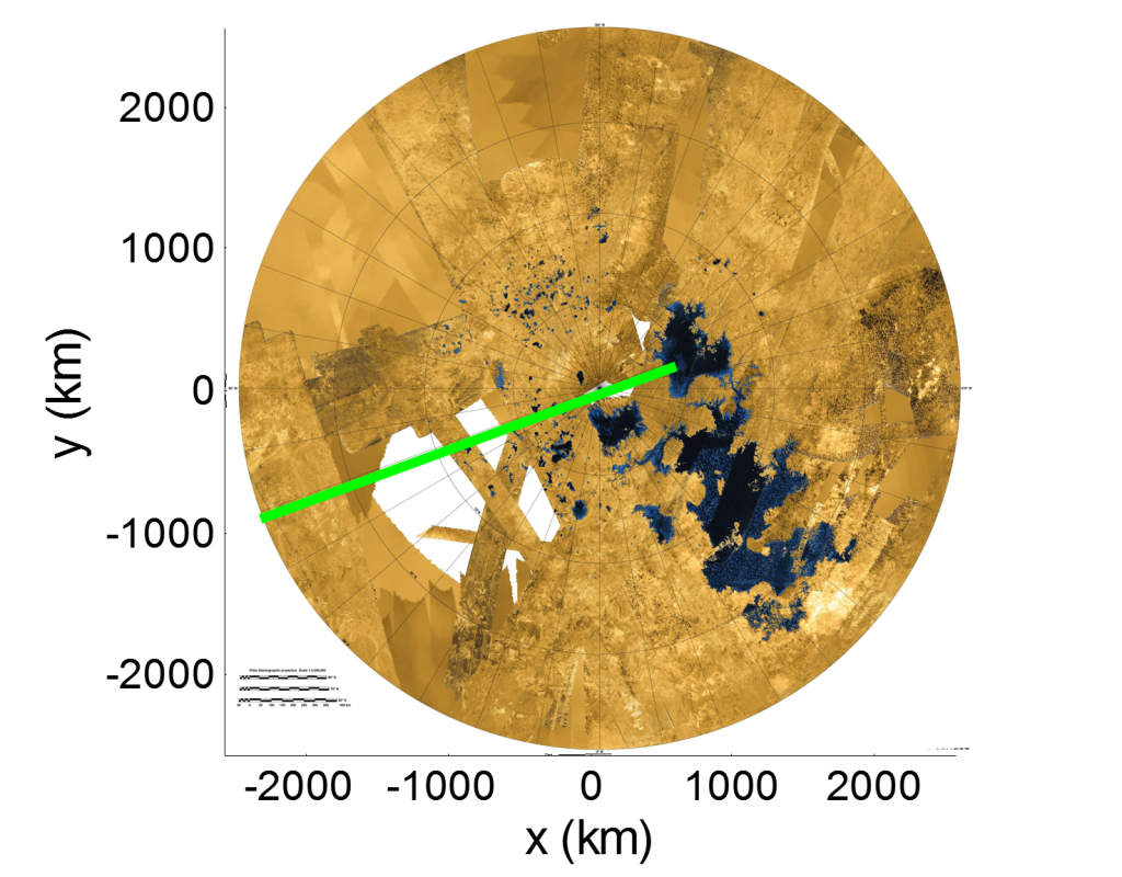
Figure 1 shows a plot of the 3D trajectory of the lander from one run of the simulation (without Monte Carlo enabled). The 2D projection of the trajectory is overlaid on a map of the North Pole of Titan, to show that landing on Ligeia Mare is possible.

Figure 2 shows the landing ellipse that the Monte Carlo simulation results in. The simulation was run about 40 times to get this distribution of data points. The drag coefficient and area of a parachute descent system were used here, and this result proved that our parachute EDL system gives us sufficient landing accuracy to guarantee a landing on Ligeia Mare.

Figure 3 provides a more visual portrayal of the landing accuracy of our parachute EDL system. The ellipse was scaled to Ligeia Mare to show that 72 km x 5 km might seem large for a landing ellipse, but is in fact quite small relative to the size of Ligeia Mare itself.

This was a really fun simulation to write and run, and there is certainly room for expansion. Including uncertainties in orbital parameters could make things interesting, as could including a thrust force in the equations of motion. After all, NASA and SpaceX are both moving towards thrust powered descent for Mars, so why not simulate it on Titan too?

References