Roshan Radhakrishnan

One of the cooler things I learned in the first half of this term is how to plot an orbit in 3D over a sphere representing the Earth. I also salvaged some old code from a friend that would project a map of the Earth over the sphere, so we can see exactly where over the Earth our spacecraft is orbiting.

What’s more, I was able to plug that code into my attitude dynamics simulator, so now the attitude dynamics simulator also plots orbital dynamics! Next step is getting a better orbit propagator in there, but I’ll have to wait for more astrodynamics theory before doing that I think. Anyways, without further ado, plots!

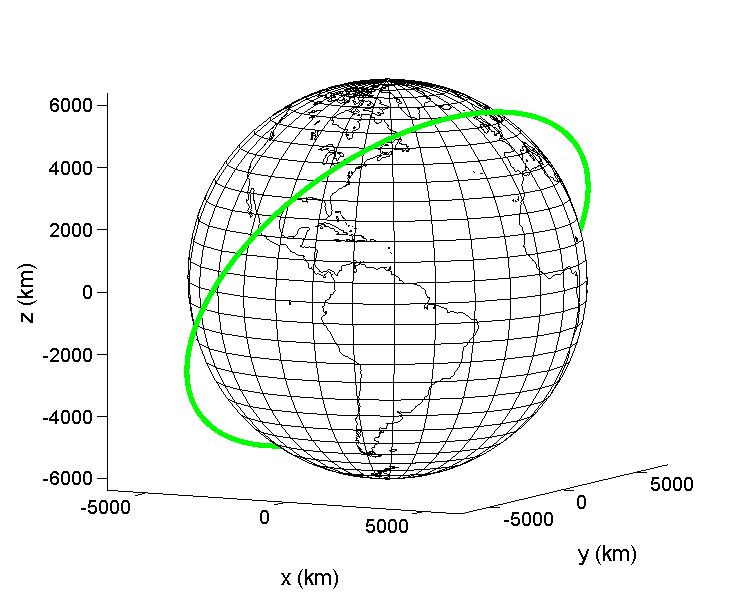
As you can see, this gorgeous plot shows us a circular orbit of a satellite passing over North America and Asia. The orbit was parameterized in the simulator by the Keplerian/classical orbital elements. The elements used for this orbit were pretty much the orbital elements describing the ISS. I made the altitude much higher though so that there was some clearer separation between the orbit and the Earth itself.

One of the most useful aspects of this type of plot is the visualization; this image allows you to get a feel for the physical meaning behind some of the orbital elements. For example, the inclination in the plot above is 51°. If we lower that to 20°, we can see the “tilt” of the orbit change below.

It is really interesting to play around with this, messing with orbital elements has given me a better intuitive understanding of them already. Getting this into the attitude dynamics simulator tonight is something I am pretty happy with, updating orbital propagation and including a drag model are probably the two biggest upgrades left. The wheel module seems to be working okay for now.  It feels good to get progress in when I didn’t expect to.

Note: I didn’t include all of the other dynamics related plots of angular velocity, quaternion, control torques, etc in this post for the sake of brevity. It’d be interesting to explore how messing with the orbit affects them though…