Roshan Radhakrishnan

I’m more hesitant to boldly declare this set of plots a success, but I do think I’m on to something decent here.

I’ve modeled the spacecraft with the same inertia properties and initial orientation and velocities that I’ve used before (found in this post). I’ve also given all the reaction wheels the same moment of inertia, 1×10^-3 kg m². This is for consistency more than anything else.

The reaction wheels are modeled as a set of three wheels with each wheel lining up with one of the spacecraft’s body frame axes. This is a very simple assumption, since it allows us to basically say that each wheel is responsible for producing one component of the control torque calculated by the control law. If the wheels were not aligned along the body frame axes, then each wheel’s spin would contribute to multiple control torque components, and we would have more involved geometry at play. In reality you would  probably have one extra wheel at an angle such that it could impart a torque about all three spacecraft body axes. That’s something I would like to model in the future. But first, baby steps.

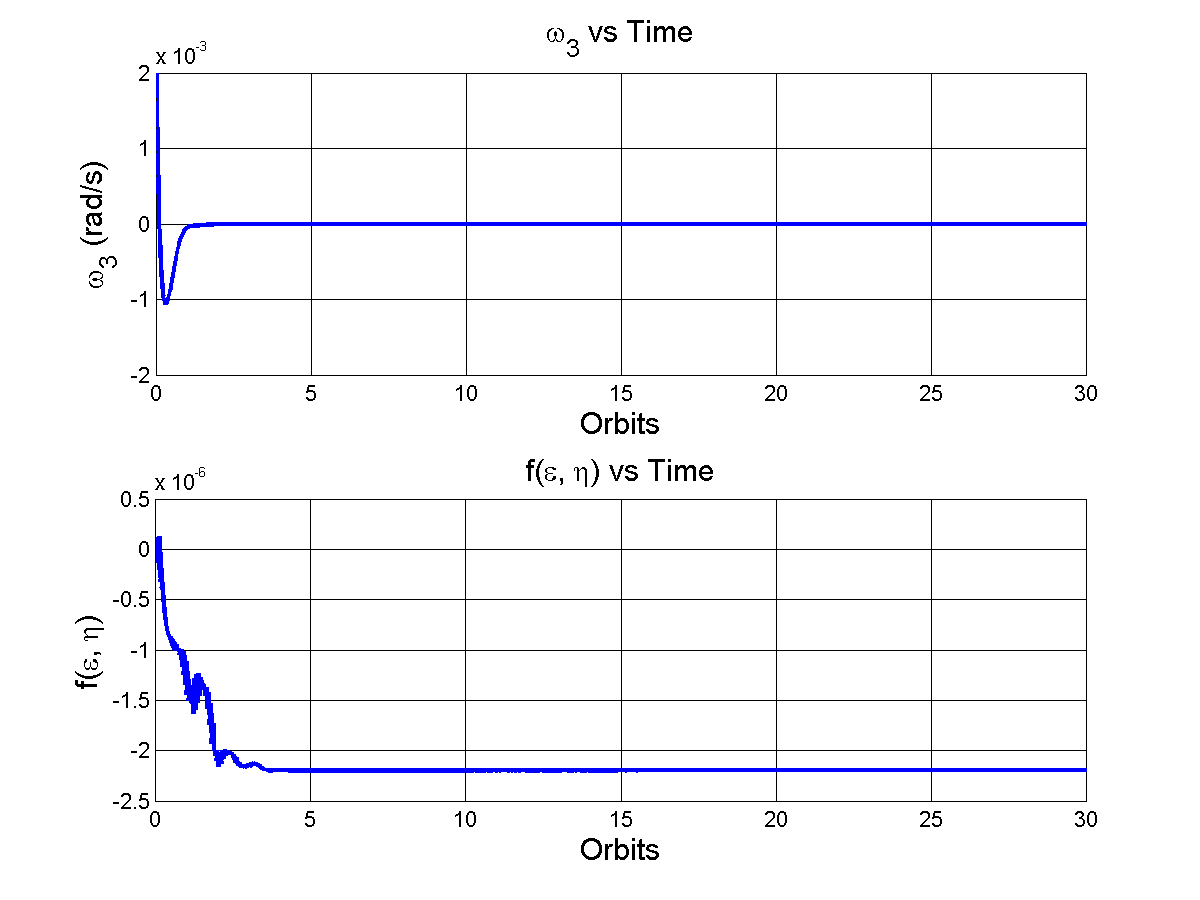
You’ll notice that when compared to the original plots with magnetic torque rods, the angular velocities and orientation settle incredibly quickly, and there is no long term oscillation. I first noticed this effect when I was doing simulations for a CubeSat project, and it had me stumped for a while.

The reason for the fantastic control here is because of one of the fundamental issues with magnetic torque rods: they depend on the Earth’s local magnetic field to generate control torques. The torque produced by a magnetic torque rod is directly proportional to the magnitude of the Earth’s magnetic field, and is also reliant on the direction of the Earth’s magnetic field. This means there is a hard mathematical barrier in effectiveness (or maximum magnitude of control torque) for torque rods. This becomes even clearer when you look at control torque plots side by side.

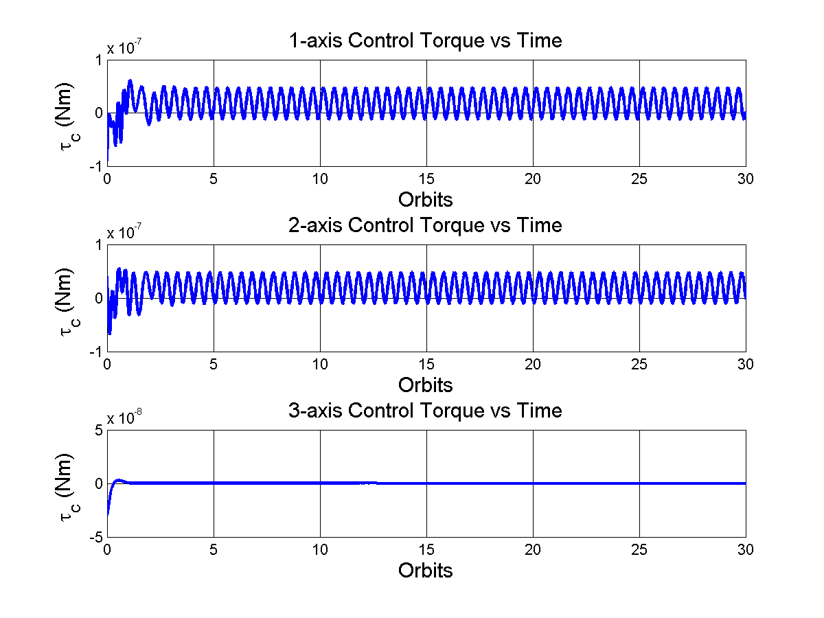
Ignoring the different plotting style I used (I’ll fix that when its not late and I don’t have class early in the morning), it is clear that the control torques produced by reaction wheels is an entire order of magnitude larger than those produced by torque rods. That is a pretty big deal, and it seems to nip both instability and long term oscillations right in the bud.

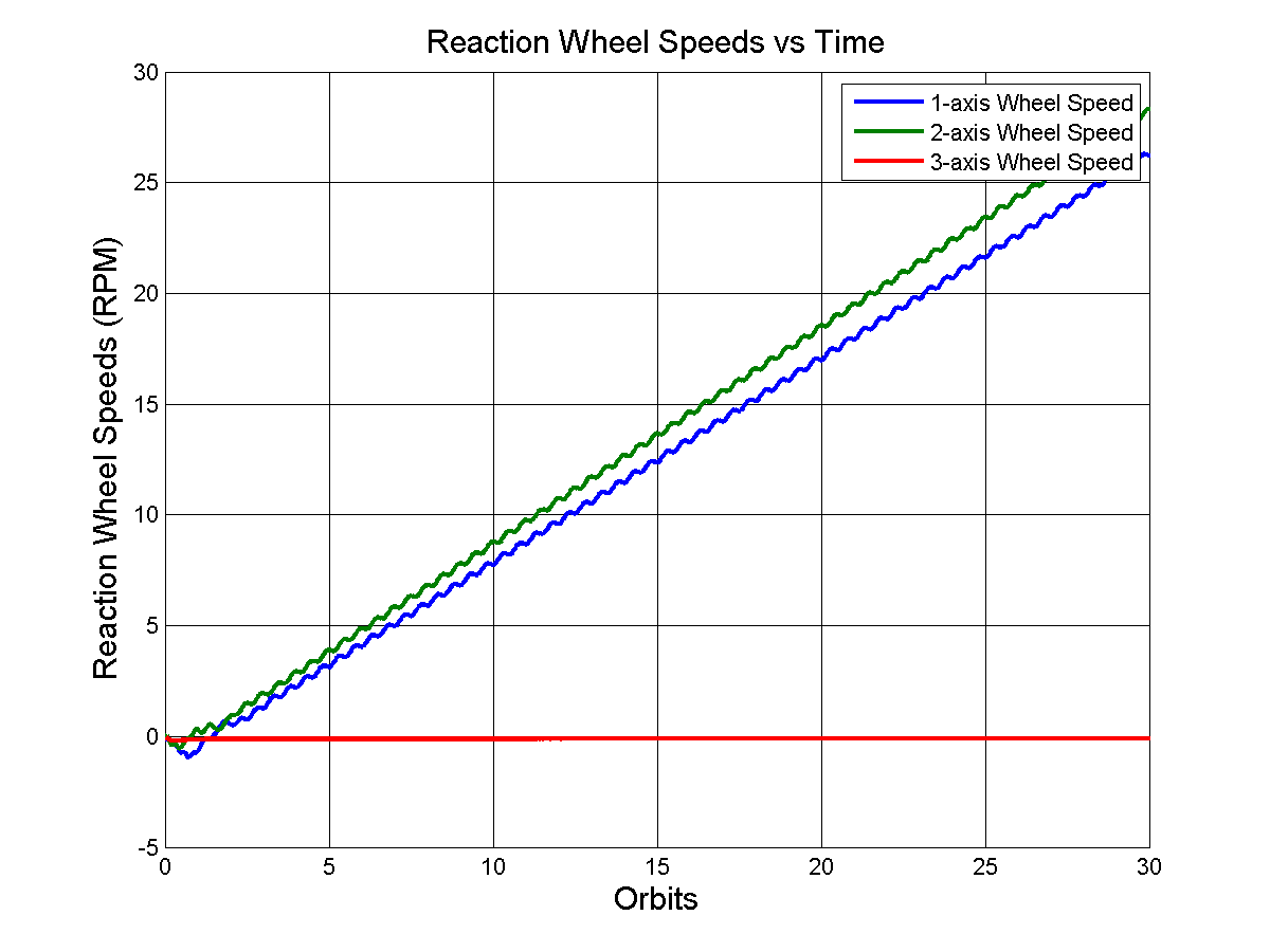
Figure 5 shows how the wheel speed about two of the three body frame axes keeps going up. This can be explained by the steady control torque required by the control law. However, this could also be due to simulation error (read: bad implementation by yours truly). I’ll have to think on this some more since I don’t completely buy the steady control torque explanation; part of me thinks the wheel speed should still level off, or not be as drastically rising. The RPMs also seem a bit low, but the plot does demonstrate one weakness of reaction wheels: saturation. A wheel can only spin up so much, according to this simulation, after around 1000 orbits (~63 days) you would have around 1000 RPM (assuming the rise stays linear) which could be a problem if your wheel only spins up to 500 RPM and you want your mission to last for a year. When a wheel hits the maximum spin rate, it has saturated, and another actuator is needed to “unload” the angular momentum stored in the wheel and bring it down to a lower spin rate. Three guesses as to what actuator is  typically used to unload angular momentum…